In this mini-project, you will explore FiveTHirtyEight’s Halloween Candy dataset.
We will use lots of ggplot some basic stats, correlation analysis and PCA to make sense of the landscape of US candy - somehting hopefully more relatable than the proteomics and transcriptomics work that we will use these methods on throughout the rest of the course
Q3. What is your favorite candy (other than Twix) in the dataset and what is it’s winpercent value?
Hershey’s Kisses’ winpercent value is 55.37545
candy["Hershey's Kisses", ]$winpercent
[1] 55.37545
Q4. What is the winpercent value for “Kit Kat”?
Kit Kat’s winpercent value is 76.7686
candy["Kit Kat", ]$winpercent
[1] 76.7686
Q5. What is the winpercent value for “Tootsie Roll Snack Bars”?
Tootsie Roll Snack Bars’ winpercent value is
candy["Tootsie Roll Snack Bars", ]$winpercent
[1] 49.6535
library("skimr")skim(candy)
Data summary
Name
candy
Number of rows
85
Number of columns
12
_______________________
Column type frequency:
numeric
12
________________________
Group variables
None
Variable type: numeric
skim_variable
n_missing
complete_rate
mean
sd
p0
p25
p50
p75
p100
hist
chocolate
0
1
0.44
0.50
0.00
0.00
0.00
1.00
1.00
▇▁▁▁▆
fruity
0
1
0.45
0.50
0.00
0.00
0.00
1.00
1.00
▇▁▁▁▆
caramel
0
1
0.16
0.37
0.00
0.00
0.00
0.00
1.00
▇▁▁▁▂
peanutyalmondy
0
1
0.16
0.37
0.00
0.00
0.00
0.00
1.00
▇▁▁▁▂
nougat
0
1
0.08
0.28
0.00
0.00
0.00
0.00
1.00
▇▁▁▁▁
crispedricewafer
0
1
0.08
0.28
0.00
0.00
0.00
0.00
1.00
▇▁▁▁▁
hard
0
1
0.18
0.38
0.00
0.00
0.00
0.00
1.00
▇▁▁▁▂
bar
0
1
0.25
0.43
0.00
0.00
0.00
0.00
1.00
▇▁▁▁▂
pluribus
0
1
0.52
0.50
0.00
0.00
1.00
1.00
1.00
▇▁▁▁▇
sugarpercent
0
1
0.48
0.28
0.01
0.22
0.47
0.73
0.99
▇▇▇▇▆
pricepercent
0
1
0.47
0.29
0.01
0.26
0.47
0.65
0.98
▇▇▇▇▆
winpercent
0
1
50.32
14.71
22.45
39.14
47.83
59.86
84.18
▃▇▆▅▂
Q6. Is there any variable/column that looks to be on a different scale to the majority of the other columns in the dataset?
“winpercent” looks to be on a different scale than the majority of the other columns. The other ones seem to be on a 0-1 scale while winpercent is not bound by those limits.
Q7. What do you think a zero and one represent for the candy$chocolate column?
In the choclolate column, a zero represents the candy not being classified as chocolate while a one means that the specific candy is classified as a chocolate type of candy.
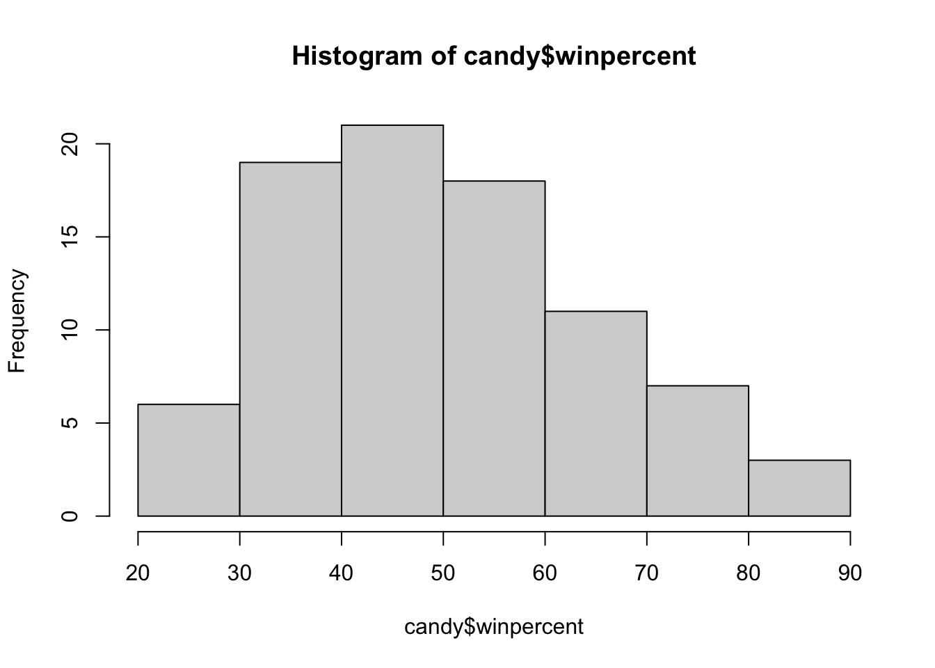
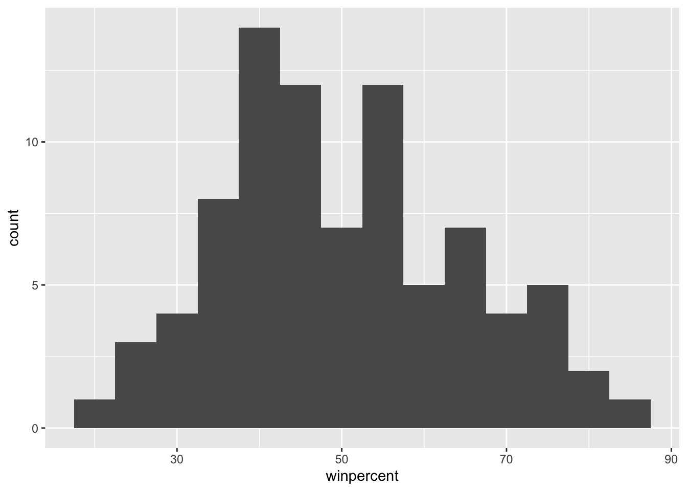
Q9. Is the distribution of winpercent values symmetrical?
No, the distribution of winpercent values is not symmetrical
Q10. Is the center of the distribution above or below 50%?
summary(candy$winpercent)
   Min. 1st Qu.  Median    Mean 3rd Qu.    Max.
  22.45   39.14   47.83   50.32   59.86   84.18
The center of the distribution depends on what you look at. If you look at the mean, it is 50.32%, which is above the threshold. If you look at the median, it is 47.83%, which is below 50%.
Q11. On average is chocolate candy higher or lower ranked than fruit candy?
    Welch Two Sample t-test

data:  chocolate and fruity
t = 6.2582, df = 68.882, p-value = 2.871e-08
alternative hypothesis: true difference in means is not equal to 0
95 percent confidence interval:
 11.44563 22.15795
sample estimates:
mean of x mean of y
 60.92153  44.11974
Yes, the means of the chocolate and fruity candy are significantly different.
Overall Candy Rankings
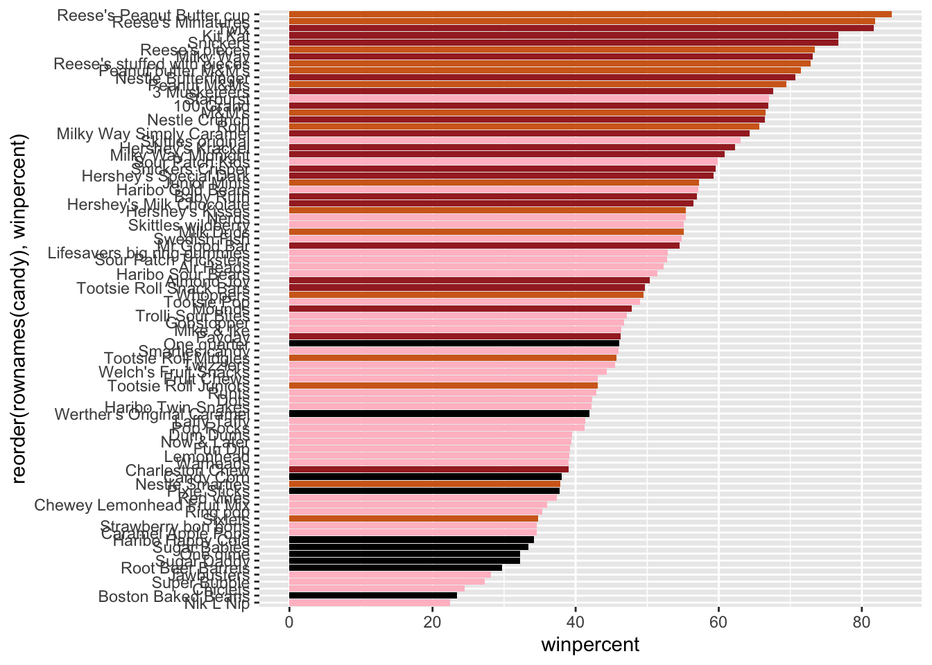
Q13. What are the five least liked candy types in this set?
head(candy[order(candy$winpercent), ], n =5)
                   chocolate fruity caramel peanutyalmondy nougat
Nik L Nip                  0      1       0              0      0
Boston Baked Beans         0      0       0              1      0
Chiclets                   0      1       0              0      0
Super Bubble               0      1       0              0      0
Jawbusters                 0      1       0              0      0
                   crispedricewafer hard bar pluribus sugarpercent pricepercent
Nik L Nip                         0    0   0        1        0.197        0.976
Boston Baked Beans                0    0   0        1        0.313        0.511
Chiclets                          0    0   0        1        0.046        0.325
Super Bubble                      0    0   0        0        0.162        0.116
Jawbusters                        0    1   0        1        0.093        0.511
                   winpercent
Nik L Nip            22.44534
Boston Baked Beans   23.41782
Chiclets             24.52499
Super Bubble         27.30386
Jawbusters           28.12744
candy |>arrange(winpercent) |>head(5)
                   chocolate fruity caramel peanutyalmondy nougat
Nik L Nip                  0      1       0              0      0
Boston Baked Beans         0      0       0              1      0
Chiclets                   0      1       0              0      0
Super Bubble               0      1       0              0      0
Jawbusters                 0      1       0              0      0
                   crispedricewafer hard bar pluribus sugarpercent pricepercent
Nik L Nip                         0    0   0        1        0.197        0.976
Boston Baked Beans                0    0   0        1        0.313        0.511
Chiclets                          0    0   0        1        0.046        0.325
Super Bubble                      0    0   0        0        0.162        0.116
Jawbusters                        0    1   0        1        0.093        0.511
                   winpercent
Nik L Nip            22.44534
Boston Baked Beans   23.41782
Chiclets             24.52499
Super Bubble         27.30386
Jawbusters           28.12744
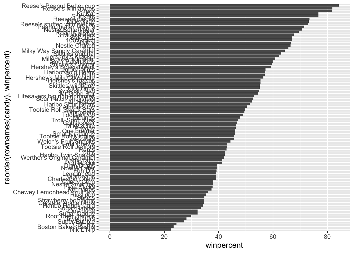
Q14. What are the top 5 all time favorite candy types out of this set?
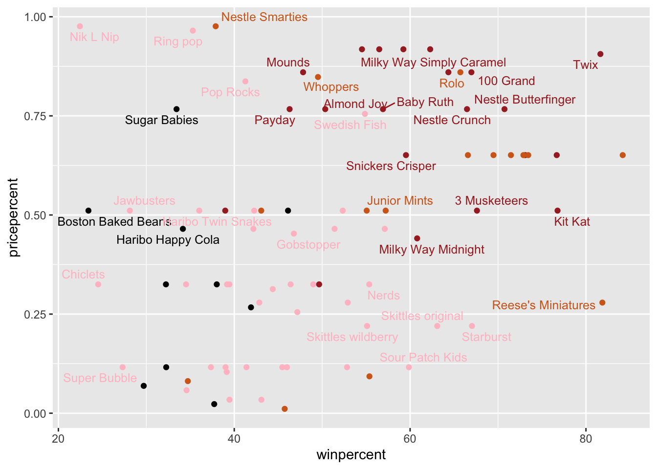
library(ggrepel)# How about a plot of win vs priceggplot(candy) +aes(winpercent, pricepercent, label=rownames(candy)) +geom_point(col=my_cols) +geom_text_repel(col=my_cols, size=3.3, max.overlaps =5)
Warning: ggrepel: 50 unlabeled data points (too many overlaps). Consider
increasing max.overlaps
Q19. Which candy type is the highest ranked in terms of winpercent for the least money - i.e. offers the most bang for your buck?
Reese’s Miniatures is the highest ranked in terms of winpercent for the least money
ord <-order(candy$winpercent, decreasing =TRUE)head( candy[ord,c(11,12)], n=5 )
Q20. What are the top 5 most expensive candy types in the dataset and of these which is the least popular?
Nik L Nip is the least popular amongst the 5 most expensive candy types.
ord <-order(candy$pricepercent, decreasing =TRUE)head( candy[ord,c(11,12)], n=5 )
                         pricepercent winpercent
Nik L Nip                       0.976   22.44534
Nestle Smarties                 0.976   37.88719
Ring pop                        0.965   35.29076
Hershey's Krackel               0.918   62.28448
Hershey's Milk Chocolate        0.918   56.49050
Optional
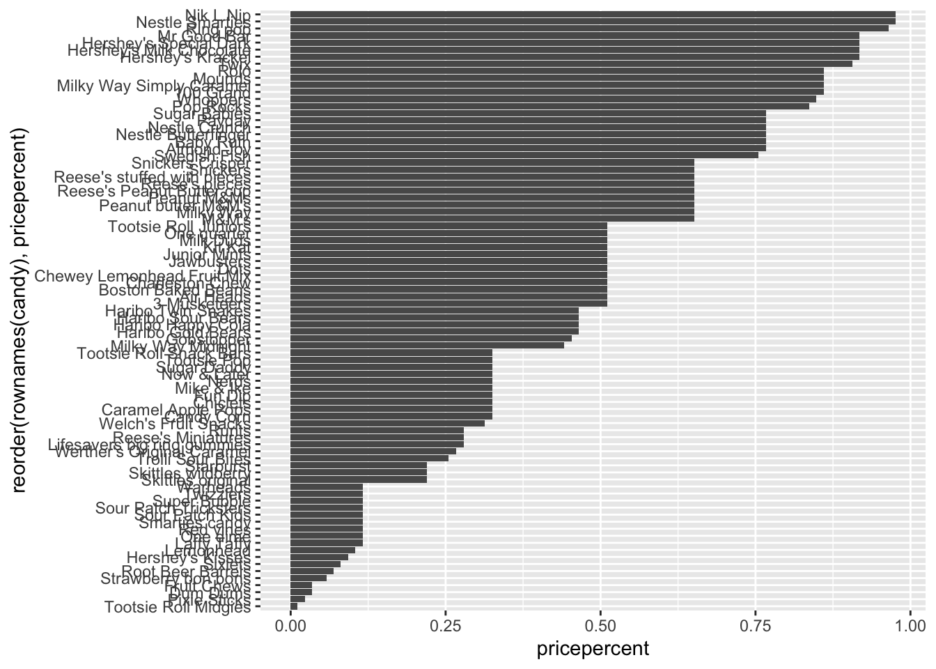
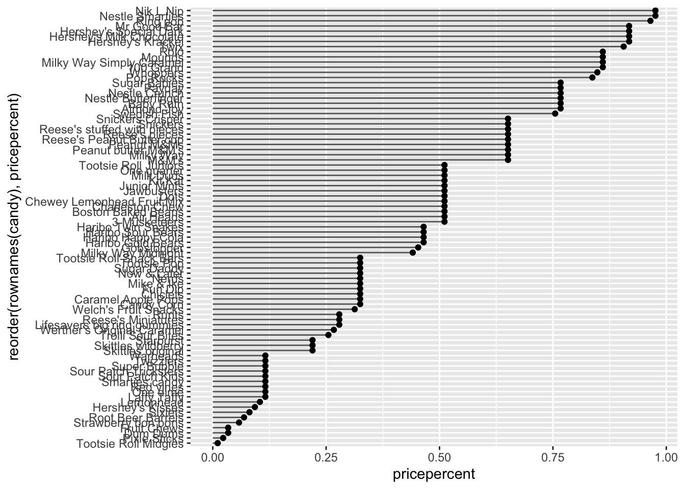
Q21. Make a barplot again with geom_col() this time using pricepercent and then improve this step by step, first ordering the x-axis by value and finally making a so called “dot chat” or “lollipop” chart by swapping geom_col() for geom_point() + geom_segment().
# Make a lollipop chart of pricepercentggplot(candy) +aes(pricepercent, reorder(rownames(candy), pricepercent)) +geom_segment(aes(yend =reorder(rownames(candy), pricepercent), xend =0), col="gray40") +geom_point()
Exploring the Correlation Structure
library(corrplot)
corrplot 0.95 loaded
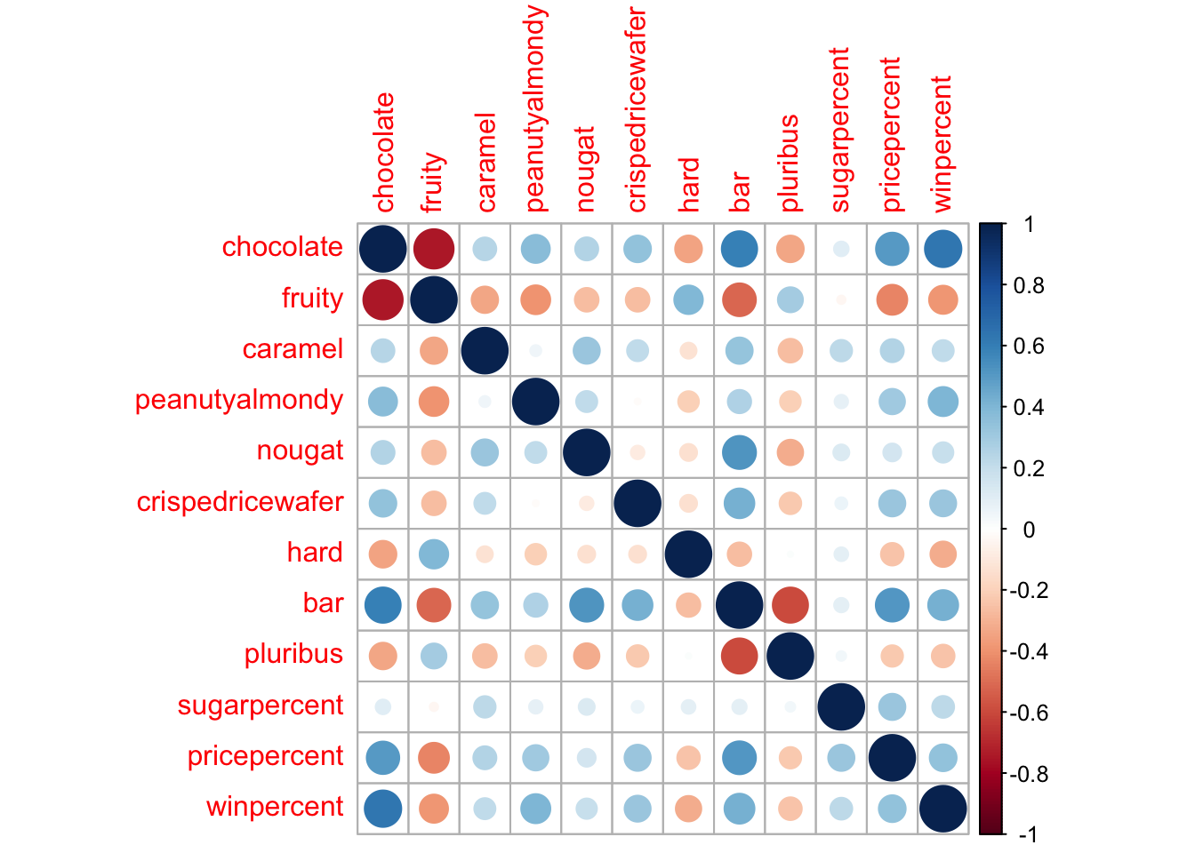
cij <-cor(candy)corrplot(cij)
Q22. Examining this plot what two variables are anti-correlated (i.e. have minus values)?
There are many variables that are anti-correlated with each other. However, Chocolate and Fruity are the two variables that are the most anti-correlated with each other.
Q23. Similarly, what two variables are most positively correlated?
Chocolate and winpercent are the two variables that are the most positively correlated.
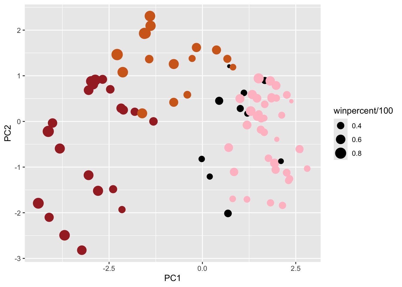
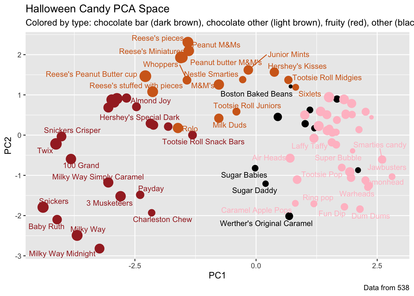
# Make a new data-frame with our PCA results and candy datamy_data <-cbind(candy, pca$x[,1:3])p <-ggplot(my_data) +aes(x=PC1, y=PC2, size=winpercent/100, text=rownames(my_data),label=rownames(my_data)) +geom_point(col=my_cols)p
library(ggrepel)p +geom_text_repel(size=3.3, col=my_cols, max.overlaps =7) +theme(legend.position ="none") +labs(title="Halloween Candy PCA Space",subtitle="Colored by type: chocolate bar (dark brown), chocolate other (light brown), fruity (red), other (black)",caption="Data from 538")
Warning: ggrepel: 39 unlabeled data points (too many overlaps). Consider
increasing max.overlaps
# library(plotly)# ggplotly(p)
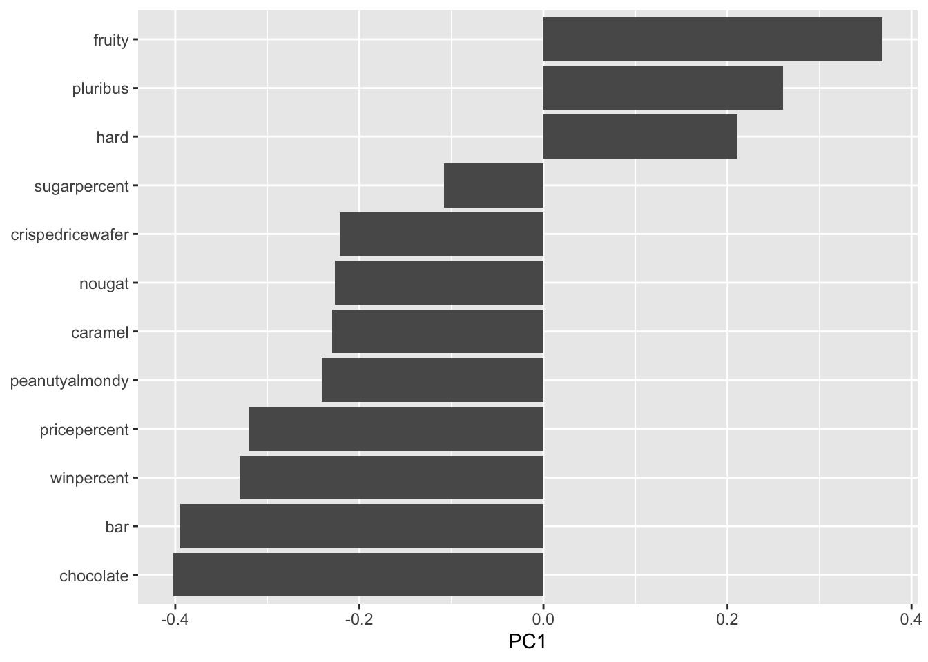
Q24. Complete the code to generate the loadings plot above. What original variables are picked up strongly by PC1 in the positive direction? Do these make sense to you? Where did you see this relationship highlighted previously?
Fruity, Pluribus, and Hard are the variables picked up strongly by PC1 in the positive direction. This makes sense because fruity and chocolate in the previous correlation plot above were the most anti-correlated with each other. If we compare fruity with the variables in the negative direction on the correlation plot, we can see that they are highly negatively correlated.
Q25. Based on your exploratory analysis, correlation findings, and PCA results, what combination of characteristics appears to make a “winning” candy? How do these different analyses (visualization, correlation, PCA) support or complement each other in reaching this conclusion?
Based on exploratory analysis, correlation findings, and PCA results, to make a “winning” candy, it generally is a chocolate with features like having a lower price point, caramel, peanutyalmondy, nougat, and a bar. These chocolate candies are correlated with a higher winpoint and thus appear to more likely to make a “winning” candy.
Optional Extension Questions
Q26. Are popular candies more expensive? In other words: is price significantly different between “winners” and “losers”? List both average values and a P-value along with your answer.
The mean of “losers” candy is 0.3744 while the mean of “winning” candies is 0.5804. The p-value is 0.0006068 which is statistically significant.This suggests that the popular candies are more expensive than the unpopular ones.
    Welch Two Sample t-test

data:  losers$pricepercent and winners$pricepercent
t = -3.5653, df = 82.798, p-value = 0.0006068
alternative hypothesis: true difference in means is not equal to 0
95 percent confidence interval:
 -0.32090727 -0.09107157
sample estimates:
mean of x mean of y
0.3743696 0.5803590
Q27. Are candies with more sugar more likely to be popular? What is your interpretation of the means and P-value in this case?
The mean of candies with more sugar is 53.949 while the mean of popular candies is 47.238 The p-value is 0.0373, which is statistically significant. This suggests that the candies with more sugar are more likely to be popular than those with less sugar.
more = candy[which(candy$sugarpercent >=0.5),]less = candy[which(candy$sugarpercent <0.5),]t.test(more$winpercent, less$winpercent)
    Welch Two Sample t-test

data:  more$winpercent and less$winpercent
t = 2.1192, df = 76.967, p-value = 0.0373
alternative hypothesis: true difference in means is not equal to 0
95 percent confidence interval:
  0.4050308 13.0167630
sample estimates:
mean of x mean of y
 53.94854  47.23765