Rows: 6 Columns: 9
── Column specification ────────────────────────────────────────────────────────
Delimiter: ","
chr (1): Molecular Type
dbl (4): Integrative, Multiple methods, Neutron, Other
num (4): X-ray, EM, NMR, Total

ℹ Use `spec()` to retrieve the full column specification for this data.
ℹ Specify the column types or set `show_col_types = FALSE` to quiet this message.
Q2: What proportion of structures in the PDB are protein?
97.91% of the structures in the PDB are proteins.
sum(stats[1:3,"Total"]) /sum(stats$Total)
[1] 0.979118
Q3: Type HIV in the PDB website search box on the home page and determine how many HIV-1 protease structures are in the current PDB?
There are currently 1173 HIV-1 protease structures in the current PDB.
Visualizing the HIV-1 Protease Structure
We can use the Molstar viewer online: https://molstar.org/viewer/
> Q4: Water molecules normally have 3 atoms. Why do we see just one atom per water molecule in this structure?
Q5: There is a critical “conserved” water molecule in the binding site. Can you identify this water molecule? What residue number does this water molecule have
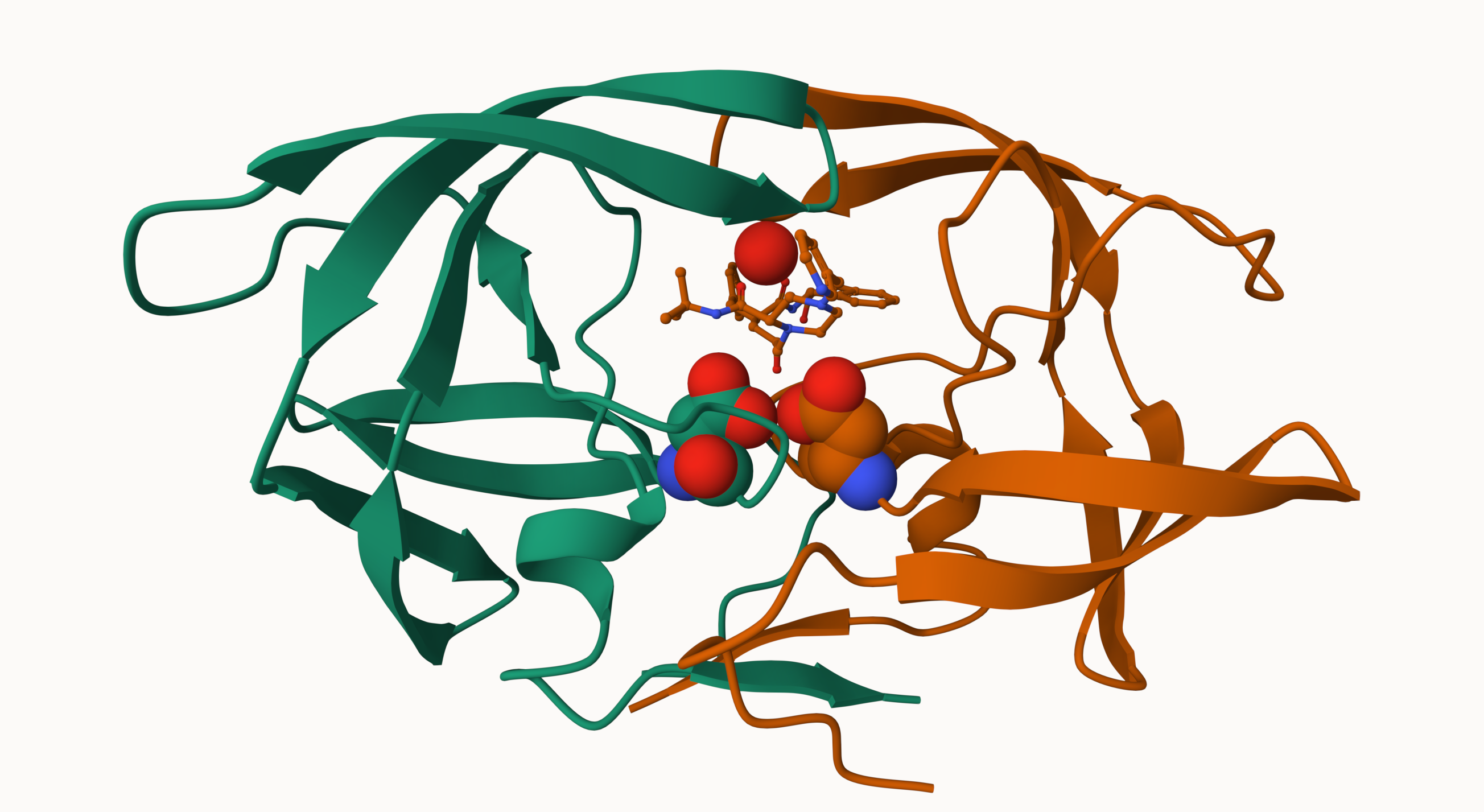
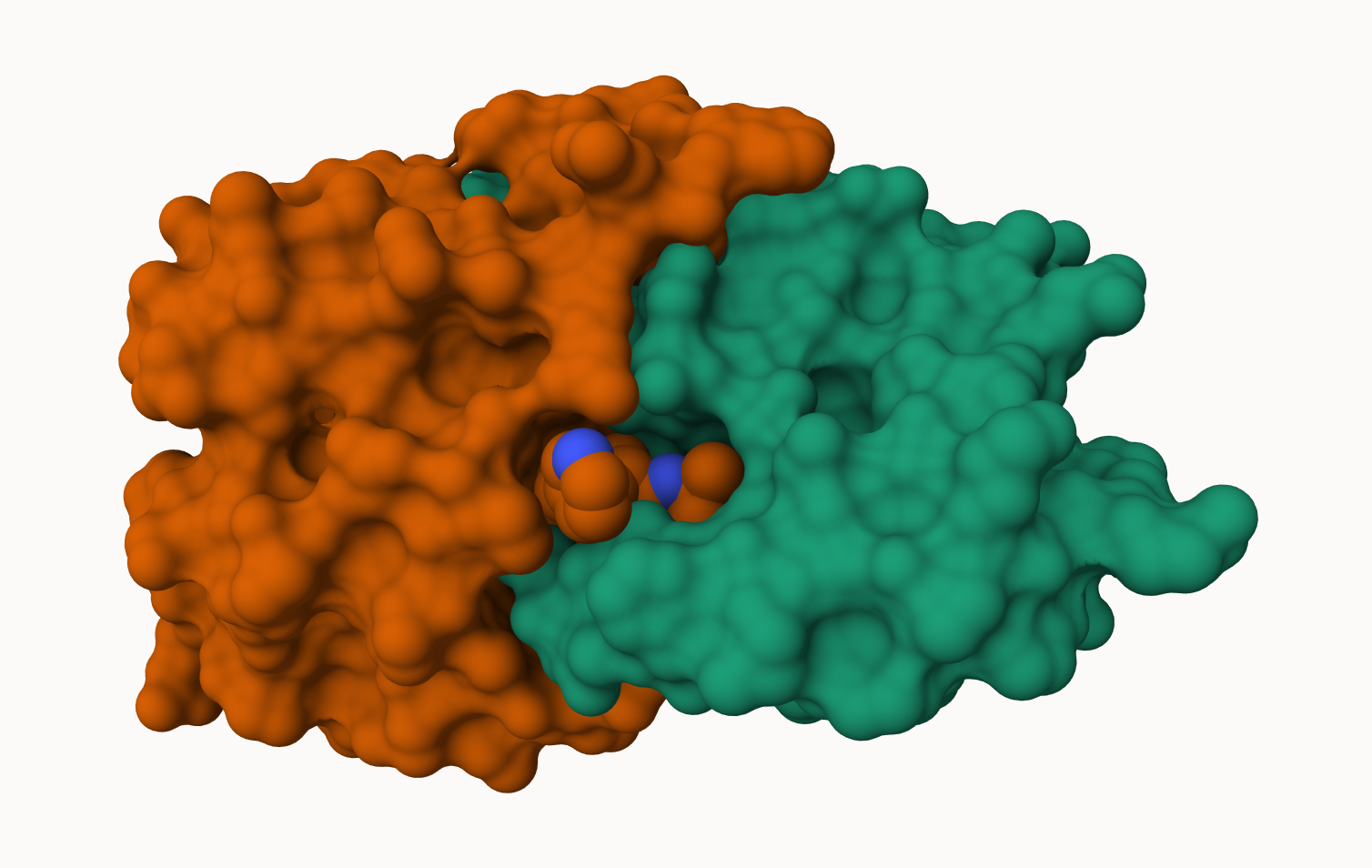
Q6: Generate and save a figure clearly showing the two distinct chains of HIV-protease along with the ligand. You might also consider showing the catalytic residues ASP 25 in each chain and the critical water (we recommend “Ball & Stick” for these side-chains). Add this figure to your Quarto document.
A new clean image showing the catalytic ASP25 amino acids in both chains of the HIV-PR dimer along with the inhibitor and all important active site water.
Q7: [Optional] As you have hopefully observed HIV protease is a homodimer (i.e. it is composed of two identical chains). With the aid of the graphic display can you identify secondary structure elements that are likely to only form in the dimer rather than the monomer?
Bio3D Package for Structural Bioinformatics
library(bio3d)pdb <-read.pdb("1hsg")
Note: Accessing on-line PDB file
pdb
 Call:  read.pdb(file = "1hsg")

   Total Models#: 1
     Total Atoms#: 1686,  XYZs#: 5058  Chains#: 2  (values: A B)

     Protein Atoms#: 1514  (residues/Calpha atoms#: 198)
     Nucleic acid Atoms#: 0  (residues/phosphate atoms#: 0)

     Non-protein/nucleic Atoms#: 172  (residues: 128)
     Non-protein/nucleic resid values: [ HOH (127), MK1 (1) ]

   Protein sequence:
      PQITLWQRPLVTIKIGGQLKEALLDTGADDTVLEEMSLPGRWKPKMIGGIGGFIKVRQYD
      QILIEICGHKAIGTVLVGPTPVNIIGRNLLTQIGCTLNFPQITLWQRPLVTIKIGGQLKE
      ALLDTGADDTVLEEMSLPGRWKPKMIGGIGGFIKVRQYDQILIEICGHKAIGTVLVGPTP
      VNIIGRNLLTQIGCTLNF

+ attr: atom, xyz, seqres, helix, sheet,
        calpha, remark, call
Q7: How many amino acid residues are there in this pdb object?
There are 198 amino acid residues in the pdb oject
Q8: Name one of the two non-protein residues?
MK1 is one of the two non-protein residues
Q9: How many protein chains are in this structure?
There are 2 protein chains in this structure
head(pdb$atom)
  type eleno elety  alt resid chain resno insert      x      y     z o     b
1 ATOM     1     N <NA>   PRO     A     1   <NA> 29.361 39.686 5.862 1 38.10
2 ATOM     2    CA <NA>   PRO     A     1   <NA> 30.307 38.663 5.319 1 40.62
3 ATOM     3     C <NA>   PRO     A     1   <NA> 29.760 38.071 4.022 1 42.64
4 ATOM     4     O <NA>   PRO     A     1   <NA> 28.600 38.302 3.676 1 43.40
5 ATOM     5    CB <NA>   PRO     A     1   <NA> 30.508 37.541 6.342 1 37.87
6 ATOM     6    CG <NA>   PRO     A     1   <NA> 29.296 37.591 7.162 1 38.40
  segid elesy charge
1  <NA>     N   <NA>
2  <NA>     C   <NA>
3  <NA>     C   <NA>
4  <NA>     O   <NA>
5  <NA>     C   <NA>
6  <NA>     C   <NA>
# Select the important ASP 25 residuesele <-atom.select(pdb, resno=25)# and highlight them in spacefill representation# view.pdb(pdb, cols=c("navy","teal"), # highlight = sele,# highlight.style = "spacefill") |># setRock()
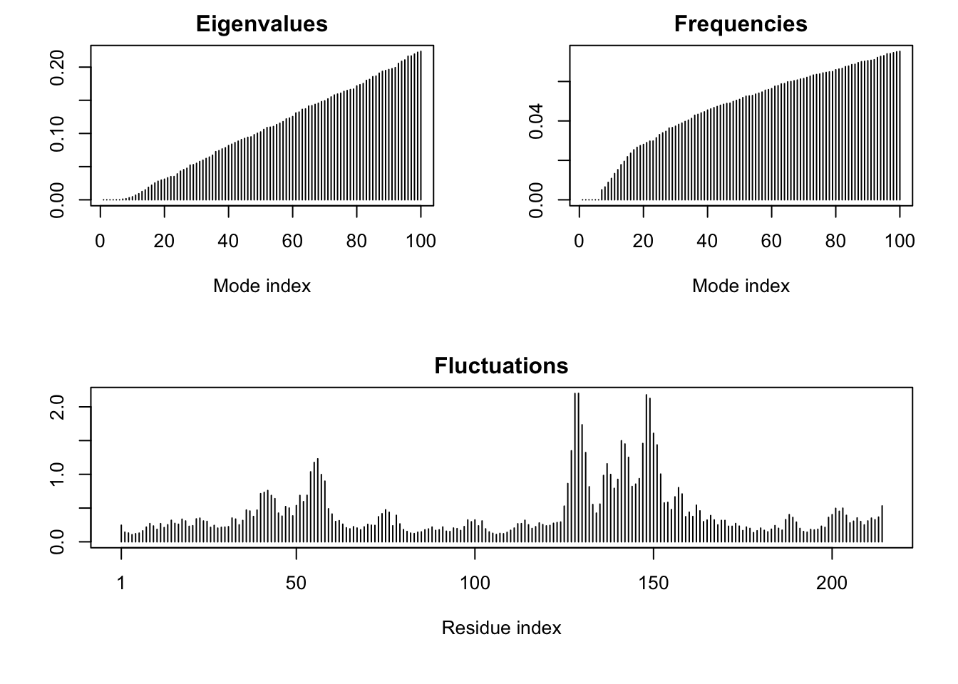
Predicting Functional Motions of a Single Structure
adk <-read.pdb("6s36")
  Note: Accessing on-line PDB file
   PDB has ALT records, taking A only, rm.alt=TRUE
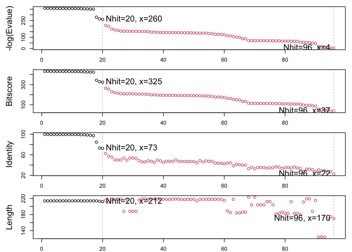
The “top hits” are in the hits object. Now we can download these to our computer. Put these in a wee sub-folder (directory) called “pdbs” and use gzip to speed things up
# Download related PDB filesfiles <-get.pdb(hits$pdb.id, path="pdbs", split=TRUE, gzip=TRUE)
Next we will use the pdbaln() function to align and also optionally fit (i.e. superpose) the identified PDB structures.
This requires a BioConductor package called “msa” that we need to install. First we install BiocManager. Then we useBiocManager::install("msa")
# Align releated PDBspdbs <-pdbaln(files, fit =TRUE, exefile="msa")
Reading PDB files:
pdbs/split_chain/1AKE_A.pdb
pdbs/split_chain/8BQF_A.pdb
pdbs/split_chain/4X8M_A.pdb
pdbs/split_chain/6S36_A.pdb
pdbs/split_chain/9R6U_A.pdb
pdbs/split_chain/9R71_A.pdb
pdbs/split_chain/8Q2B_A.pdb
pdbs/split_chain/8RJ9_A.pdb
pdbs/split_chain/6RZE_A.pdb
pdbs/split_chain/4X8H_A.pdb
pdbs/split_chain/3HPR_A.pdb
pdbs/split_chain/1E4V_A.pdb
pdbs/split_chain/5EJE_A.pdb
pdbs/split_chain/1E4Y_A.pdb
pdbs/split_chain/3X2S_A.pdb
pdbs/split_chain/6HAP_A.pdb
pdbs/split_chain/6HAM_A.pdb
pdbs/split_chain/8PVW_A.pdb
pdbs/split_chain/4K46_A.pdb
pdbs/split_chain/4NP6_A.pdb
   PDB has ALT records, taking A only, rm.alt=TRUE
.   PDB has ALT records, taking A only, rm.alt=TRUE
..   PDB has ALT records, taking A only, rm.alt=TRUE
.   PDB has ALT records, taking A only, rm.alt=TRUE
.   PDB has ALT records, taking A only, rm.alt=TRUE
.   PDB has ALT records, taking A only, rm.alt=TRUE
.   PDB has ALT records, taking A only, rm.alt=TRUE
.   PDB has ALT records, taking A only, rm.alt=TRUE
..   PDB has ALT records, taking A only, rm.alt=TRUE
..   PDB has ALT records, taking A only, rm.alt=TRUE
....   PDB has ALT records, taking A only, rm.alt=TRUE
.   PDB has ALT records, taking A only, rm.alt=TRUE
.   PDB has ALT records, taking A only, rm.alt=TRUE
..

Extracting sequences

pdb/seq: 1   name: pdbs/split_chain/1AKE_A.pdb
   PDB has ALT records, taking A only, rm.alt=TRUE
pdb/seq: 2   name: pdbs/split_chain/8BQF_A.pdb
   PDB has ALT records, taking A only, rm.alt=TRUE
pdb/seq: 3   name: pdbs/split_chain/4X8M_A.pdb
pdb/seq: 4   name: pdbs/split_chain/6S36_A.pdb
   PDB has ALT records, taking A only, rm.alt=TRUE
pdb/seq: 5   name: pdbs/split_chain/9R6U_A.pdb
   PDB has ALT records, taking A only, rm.alt=TRUE
pdb/seq: 6   name: pdbs/split_chain/9R71_A.pdb
   PDB has ALT records, taking A only, rm.alt=TRUE
pdb/seq: 7   name: pdbs/split_chain/8Q2B_A.pdb
   PDB has ALT records, taking A only, rm.alt=TRUE
pdb/seq: 8   name: pdbs/split_chain/8RJ9_A.pdb
   PDB has ALT records, taking A only, rm.alt=TRUE
pdb/seq: 9   name: pdbs/split_chain/6RZE_A.pdb
   PDB has ALT records, taking A only, rm.alt=TRUE
pdb/seq: 10   name: pdbs/split_chain/4X8H_A.pdb
pdb/seq: 11   name: pdbs/split_chain/3HPR_A.pdb
   PDB has ALT records, taking A only, rm.alt=TRUE
pdb/seq: 12   name: pdbs/split_chain/1E4V_A.pdb
pdb/seq: 13   name: pdbs/split_chain/5EJE_A.pdb
   PDB has ALT records, taking A only, rm.alt=TRUE
pdb/seq: 14   name: pdbs/split_chain/1E4Y_A.pdb
pdb/seq: 15   name: pdbs/split_chain/3X2S_A.pdb
pdb/seq: 16   name: pdbs/split_chain/6HAP_A.pdb
pdb/seq: 17   name: pdbs/split_chain/6HAM_A.pdb
   PDB has ALT records, taking A only, rm.alt=TRUE
pdb/seq: 18   name: pdbs/split_chain/8PVW_A.pdb
   PDB has ALT records, taking A only, rm.alt=TRUE
pdb/seq: 19   name: pdbs/split_chain/4K46_A.pdb
   PDB has ALT records, taking A only, rm.alt=TRUE
pdb/seq: 20   name: pdbs/split_chain/4NP6_A.pdb
Have a wee peek at this new “alignment object” pdbs
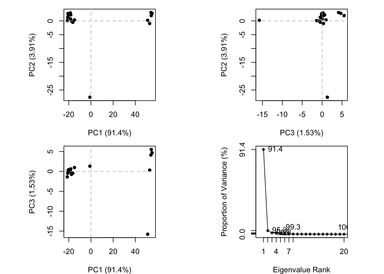
We can run PCA on our pdbs object using the pca() function from bio3d:
pc.xray <-pca(pdbs)plot(pc.xray)
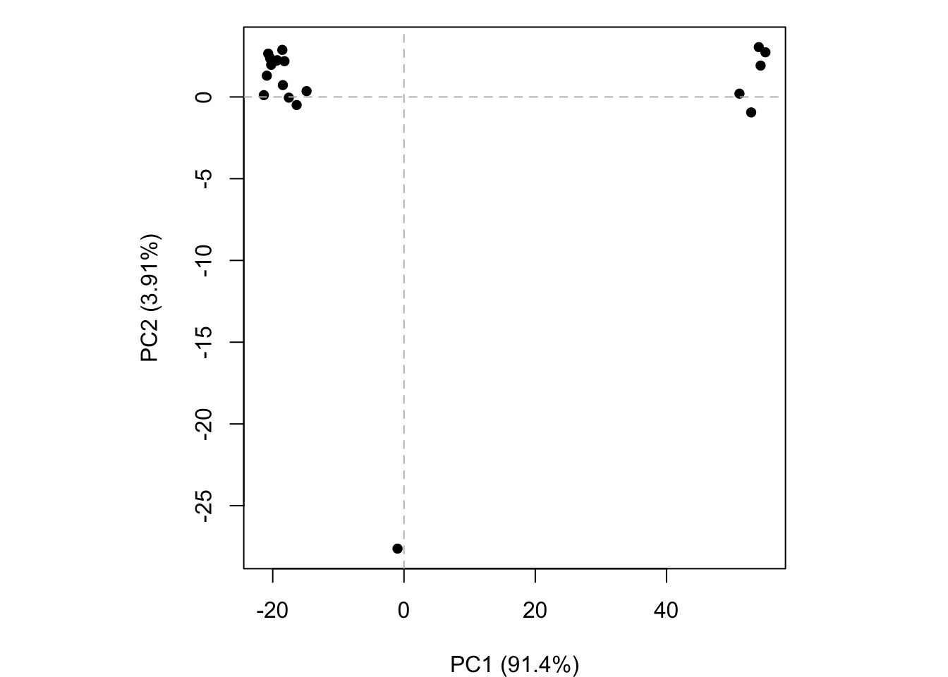
plot(pc.xray, 1:2)
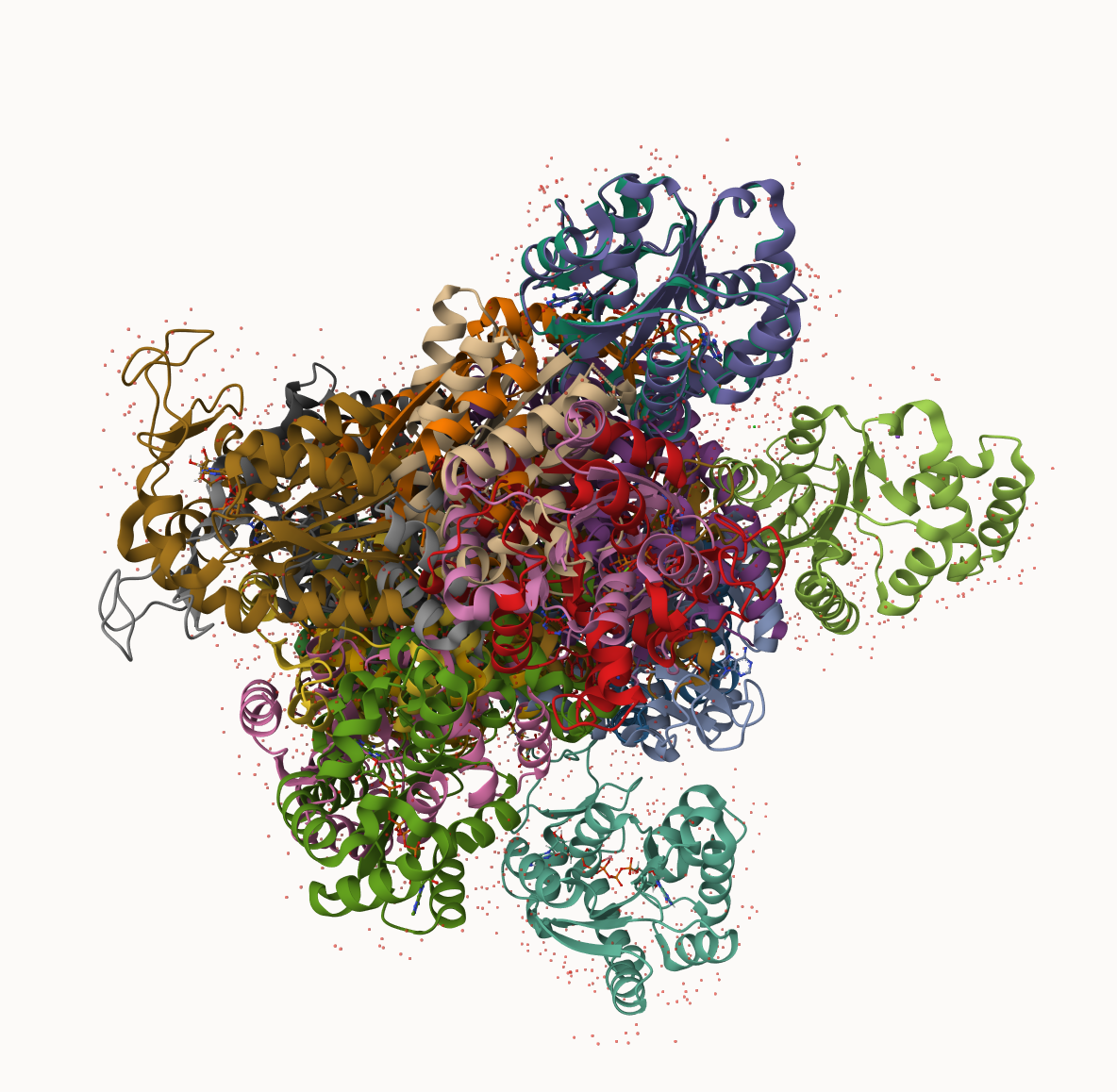
We can make a visualization of the major conformational difference (i.e. large scale structure change) captured by our PCA analysis with the mktrj() function.
 > Q4: Water molecules normally have 3 atoms. Why do we see just one atom per water molecule in this structure?