Class 11

Background

We saw last day that the main repository for biomolecular structure (the PDB database) only has ~250,000 entries.

UnitProtKB (the main protein sequence database) has over 200 million entries!

AlphaFold

In this hands-on session we will utilize AlphaFold to predict protein structure from sequence (Jumper et al. 2021).

Without the aid of such approaches, it can take years of expensive laboratory work to determine the structure of just one protein. With AlphaFold we can now accurately compute a typical protein structure in as little as ten minutes.

This major breakthrough (Figure 1) promises to place Molecular Biology in a new era where we can visualize, analyze and interpret the structures and functions of all proteins.

The EBI AlphaFold Database

The EBI AlphaFold database contains lots of computed structure models. It is increasingly likely that the strucutre you are interested in is already in this database at < https://alphafold.ebi.ac.uk/ >

There are 3 major outputs from AlphaFold

1. A model of structure in PDB format
2. a pLDDT score: that tells us how confident the model is for a given residue in your protein (High values are good, above 70)
3. a PAE score that tells us about protein packing quality

If you can’t find a matching entry for the sequence you are interested in AFDB, you can run AlphaFold yourself…

Running AlphaFold

We will use ColabFold to run AlphaFold on our sequence < https://colab.research.google.com/github/sokrypton/ColabFold/ >

Figure from AlphaFold Here!

Interpreting Results

Custom analysis of resulting models

We can read all the AlphaFold results in to R and do more quantitative analysis than just viewing the structures in Mol-star:

Read all the PDB models:

library(bio3d)

# File names for all PDB models
pdb_files <- list.files("hivpr_23119/", pattern = ".pdb", full.names = TRUE)

# Print our PDB file names
basename(pdb_files)

[1] "hivpr_23119_unrelaxed_rank_001_alphafold2_multimer_v3_model_4_seed_000.pdb"
[2] "hivpr_23119_unrelaxed_rank_002_alphafold2_multimer_v3_model_1_seed_000.pdb"
[3] "hivpr_23119_unrelaxed_rank_003_alphafold2_multimer_v3_model_5_seed_000.pdb"
[4] "hivpr_23119_unrelaxed_rank_004_alphafold2_multimer_v3_model_2_seed_000.pdb"
[5] "hivpr_23119_unrelaxed_rank_005_alphafold2_multimer_v3_model_3_seed_000.pdb"

# Read all data from Models 
#  and superpose/fit coords
pdbs <- pdbaln(pdb_files, fit=TRUE, exefile="msa")

Reading PDB files:
hivpr_23119//hivpr_23119_unrelaxed_rank_001_alphafold2_multimer_v3_model_4_seed_000.pdb
hivpr_23119//hivpr_23119_unrelaxed_rank_002_alphafold2_multimer_v3_model_1_seed_000.pdb
hivpr_23119//hivpr_23119_unrelaxed_rank_003_alphafold2_multimer_v3_model_5_seed_000.pdb
hivpr_23119//hivpr_23119_unrelaxed_rank_004_alphafold2_multimer_v3_model_2_seed_000.pdb
hivpr_23119//hivpr_23119_unrelaxed_rank_005_alphafold2_multimer_v3_model_3_seed_000.pdb
.....

Extracting sequences

pdb/seq: 1   name: hivpr_23119//hivpr_23119_unrelaxed_rank_001_alphafold2_multimer_v3_model_4_seed_000.pdb 
pdb/seq: 2   name: hivpr_23119//hivpr_23119_unrelaxed_rank_002_alphafold2_multimer_v3_model_1_seed_000.pdb 
pdb/seq: 3   name: hivpr_23119//hivpr_23119_unrelaxed_rank_003_alphafold2_multimer_v3_model_5_seed_000.pdb 
pdb/seq: 4   name: hivpr_23119//hivpr_23119_unrelaxed_rank_004_alphafold2_multimer_v3_model_2_seed_000.pdb 
pdb/seq: 5   name: hivpr_23119//hivpr_23119_unrelaxed_rank_005_alphafold2_multimer_v3_model_3_seed_000.pdb 

# library(bio3dview)
# view.pdbs(pdbs)

How similar or different are my models?

rd <- rmsd(pdbs)

Warning in rmsd(pdbs): No indices provided, using the 198 non NA positions

library(pheatmap)

colnames(rd) <- paste0("m",1:5)
rownames(rd) <- paste0("m",1:5)
pheatmap(rd)

Now lets plot the pLDDT values across all models.

# Read a reference PDB structure
pdb <- read.pdb("1hsg")

  Note: Accessing on-line PDB file

plotb3(pdbs$b[1,], typ="l", lwd=2, sse=pdb)
points(pdbs$b[2,], typ="l", col="red")
points(pdbs$b[3,], typ="l", col="blue")
points(pdbs$b[4,], typ="l", col="darkgreen")
points(pdbs$b[5,], typ="l", col="orange")
abline(v=100, col="gray")

We can improve the superposition/fitting of our models by finding the most consistent “rigid core” common across all the models. For this we will use the core.find() function:

core <- core.find(pdbs)

 core size 197 of 198  vol = 5310.035 
 core size 196 of 198  vol = 4635.834 
 core size 195 of 198  vol = 1812.524 
 core size 194 of 198  vol = 1109.016 
 core size 193 of 198  vol = 1035.296 
 core size 192 of 198  vol = 986.96 
 core size 191 of 198  vol = 941.365 
 core size 190 of 198  vol = 898.466 
 core size 189 of 198  vol = 857.922 
 core size 188 of 198  vol = 824.025 
 core size 187 of 198  vol = 793.081 
 core size 186 of 198  vol = 763.85 
 core size 185 of 198  vol = 740.429 
 core size 184 of 198  vol = 700.174 
 core size 183 of 198  vol = 673.821 
 core size 182 of 198  vol = 652.067 
 core size 181 of 198  vol = 634.066 
 core size 180 of 198  vol = 616.025 
 core size 179 of 198  vol = 599.771 
 core size 178 of 198  vol = 583.741 
 core size 177 of 198  vol = 568.863 
 core size 176 of 198  vol = 554.38 
 core size 175 of 198  vol = 536.073 
 core size 174 of 198  vol = 524.642 
 core size 173 of 198  vol = 510.527 
 core size 172 of 198  vol = 482.586 
 core size 171 of 198  vol = 464.833 
 core size 170 of 198  vol = 451.199 
 core size 169 of 198  vol = 435.724 
 core size 168 of 198  vol = 422.476 
 core size 167 of 198  vol = 412.705 
 core size 166 of 198  vol = 400.321 
 core size 165 of 198  vol = 389.367 
 core size 164 of 198  vol = 375.984 
 core size 163 of 198  vol = 364.58 
 core size 162 of 198  vol = 350.368 
 core size 161 of 198  vol = 338.444 
 core size 160 of 198  vol = 326.536 
 core size 159 of 198  vol = 315.655 
 core size 158 of 198  vol = 303.764 
 core size 157 of 198  vol = 292.94 
 core size 156 of 198  vol = 281.907 
 core size 155 of 198  vol = 272.908 
 core size 154 of 198  vol = 263.955 
 core size 153 of 198  vol = 254.522 
 core size 152 of 198  vol = 245.239 
 core size 151 of 198  vol = 231.669 
 core size 150 of 198  vol = 219.592 
 core size 149 of 198  vol = 211.974 
 core size 148 of 198  vol = 204.299 
 core size 147 of 198  vol = 194.165 
 core size 146 of 198  vol = 186.442 
 core size 145 of 198  vol = 178.703 
 core size 144 of 198  vol = 170.526 
 core size 143 of 198  vol = 163.019 
 core size 142 of 198  vol = 152.8 
 core size 141 of 198  vol = 143.077 
 core size 140 of 198  vol = 137.043 
 core size 139 of 198  vol = 131.686 
 core size 138 of 198  vol = 124.269 
 core size 137 of 198  vol = 117.206 
 core size 136 of 198  vol = 111.441 
 core size 135 of 198  vol = 104.8 
 core size 134 of 198  vol = 98.704 
 core size 133 of 198  vol = 94.662 
 core size 132 of 198  vol = 90.487 
 core size 131 of 198  vol = 87.458 
 core size 130 of 198  vol = 83.811 
 core size 129 of 198  vol = 79.337 
 core size 128 of 198  vol = 75.465 
 core size 127 of 198  vol = 71.717 
 core size 126 of 198  vol = 68.457 
 core size 125 of 198  vol = 64.79 
 core size 124 of 198  vol = 62.058 
 core size 123 of 198  vol = 58.244 
 core size 122 of 198  vol = 54.043 
 core size 121 of 198  vol = 49.43 
 core size 120 of 198  vol = 46.72 
 core size 119 of 198  vol = 43.468 
 core size 118 of 198  vol = 40 
 core size 117 of 198  vol = 37.229 
 core size 116 of 198  vol = 34.353 
 core size 115 of 198  vol = 31.473 
 core size 114 of 198  vol = 28.779 
 core size 113 of 198  vol = 26.188 
 core size 112 of 198  vol = 24.174 
 core size 111 of 198  vol = 22.314 
 core size 110 of 198  vol = 20.553 
 core size 109 of 198  vol = 18.935 
 core size 108 of 198  vol = 17.265 
 core size 107 of 198  vol = 15.517 
 core size 106 of 198  vol = 13.676 
 core size 105 of 198  vol = 12.402 
 core size 104 of 198  vol = 11.182 
 core size 103 of 198  vol = 10.242 
 core size 102 of 198  vol = 8.928 
 core size 101 of 198  vol = 8.18 
 core size 100 of 198  vol = 7.219 
 core size 99 of 198  vol = 6.1 
 core size 98 of 198  vol = 5.264 
 core size 97 of 198  vol = 4.359 
 core size 96 of 198  vol = 3.772 
 core size 95 of 198  vol = 3.183 
 core size 94 of 198  vol = 2.696 
 core size 93 of 198  vol = 2.414 
 core size 92 of 198  vol = 1.876 
 core size 91 of 198  vol = 1.611 
 core size 90 of 198  vol = 1.272 
 core size 89 of 198  vol = 1.038 
 core size 88 of 198  vol = 0.857 
 core size 87 of 198  vol = 0.686 
 core size 86 of 198  vol = 0.54 
 core size 85 of 198  vol = 0.44 
 FINISHED: Min vol ( 0.5 ) reached

# We can now use the identified core atom positions as a basis for a more suitable superposition and write out the fitted structures to a directory called corefit_structures
core.inds <- print(core, vol=0.5)

# 86 positions (cumulative volume <= 0.5 Angstrom^3) 
  start end length
1     9  50     42
2    52  95     44

xyz <- pdbfit(pdbs, core.inds, outpath="corefit_structures")

Now we can examine the RMSF between positions of the structure. RMSF is an often used measure of conformational variance along the structure:

rf <- rmsf(xyz)

plotb3(rf, sse=pdb)
abline(v=100, col="gray", ylab="RMSF")

Predicted Alignment Error for Domains (PAE):

library(jsonlite)

# Listing of all PAE JSON files
pae_files <- list.files("hivpr_23119/",
                        pattern=".*model.*\\.json",
                        full.names = TRUE)

pae1 <- read_json(pae_files[1],simplifyVector = TRUE)
pae5 <- read_json(pae_files[5],simplifyVector = TRUE)

attributes(pae1)

$names
[1] "plddt"   "max_pae" "pae"     "ptm"     "iptm"   

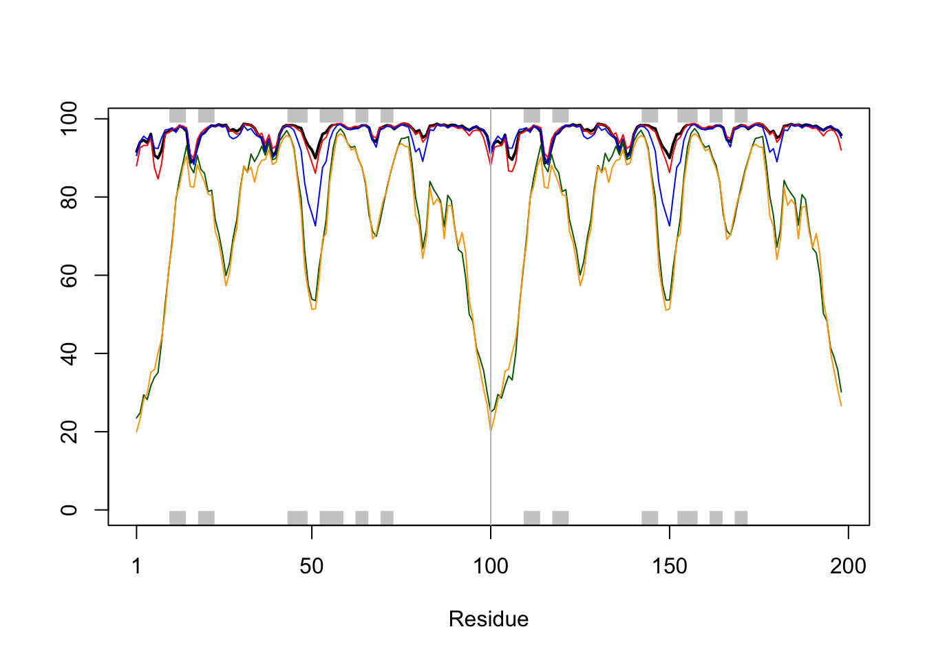
# Per-residue pLDDT scores 
#  same as B-factor of PDB..
head(pae1$plddt) 

[1] 91.62 94.06 94.56 93.88 96.12 90.69

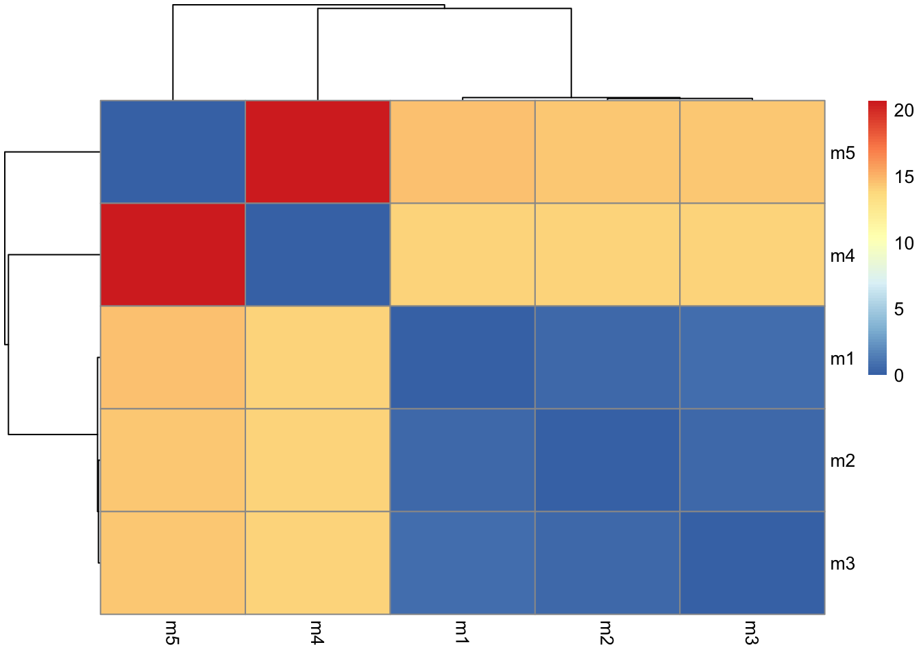
The maximum PAE values are useful for ranking models. Here we can see that model 5 is much worse than model 1. The lower the PAE score the better. How about the other models, what are thir max PAE scores?

pae1$max_pae

[1] 12.33594

pae5$max_pae

[1] 29.45312

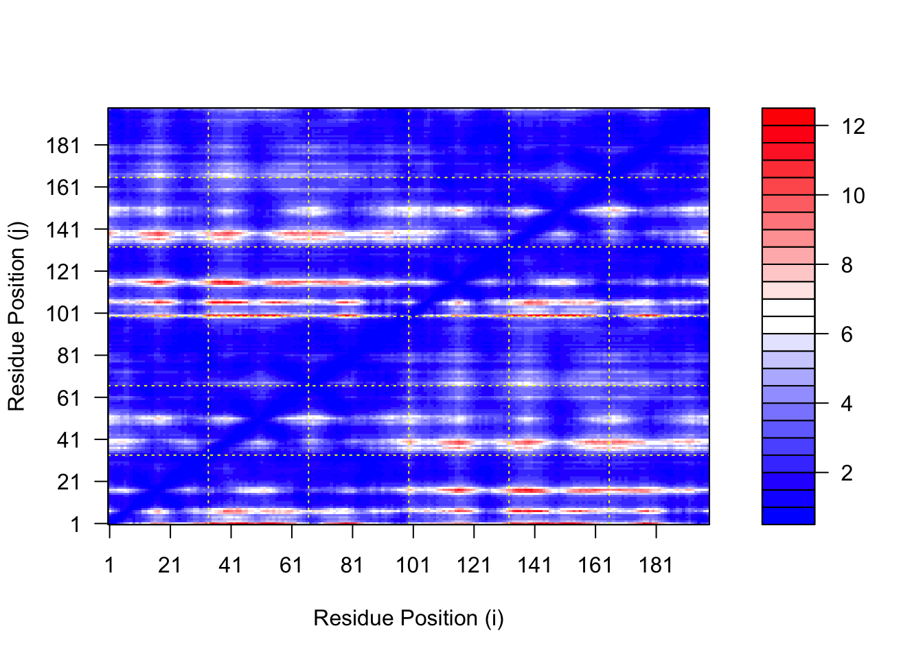
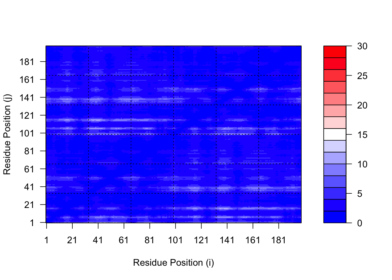
We can plot the N by N (where N is the number of residues) PAE scores with ggplot or with functions from the Bio3D package:

plot.dmat(pae1$pae, 
          xlab="Residue Position (i)",
          ylab="Residue Position (j)")

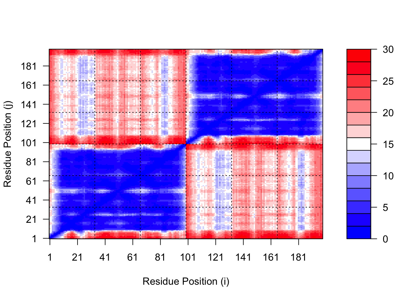
plot.dmat(pae5$pae, 
          xlab="Residue Position (i)",
          ylab="Residue Position (j)",
          grid.col = "black",
          zlim=c(0,30))

We should really plot all of these using the same z range. Here is the model 1 plot again but this time using the same data range as the plot for model 5:

plot.dmat(pae1$pae, 
          xlab="Residue Position (i)",
          ylab="Residue Position (j)",
          grid.col = "black",
          zlim=c(0,30))

Residue Conservation from Alignment File

aln_file <- list.files("hivpr_23119/",
                       pattern=".a3m$",
                        full.names = TRUE)
aln_file

[1] "hivpr_23119//hivpr_23119.a3m"

aln <- read.fasta(aln_file[1], to.upper = TRUE)

[1] " ** Duplicated sequence id's: 101 **"
[2] " ** Duplicated sequence id's: 101 **"

dim(aln$ali)

[1] 5397  132

We can score residue conservation in the alignment with the conserv() function.

sim <- conserv(aln)

plotb3(sim[1:99], sse=trim.pdb(pdb, chain="A"),
       ylab="Conservation Score")

con <- consensus(aln, cutoff = 0.9)
con$seq

  [1] "-" "-" "-" "-" "-" "-" "-" "-" "-" "-" "-" "-" "-" "-" "-" "-" "-" "-"
 [19] "-" "-" "-" "-" "-" "-" "D" "T" "G" "A" "-" "-" "-" "-" "-" "-" "-" "-"
 [37] "-" "-" "-" "-" "-" "-" "-" "-" "-" "-" "-" "-" "-" "-" "-" "-" "-" "-"
 [55] "-" "-" "-" "-" "-" "-" "-" "-" "-" "-" "-" "-" "-" "-" "-" "-" "-" "-"
 [73] "-" "-" "-" "-" "-" "-" "-" "-" "-" "-" "-" "-" "-" "-" "-" "-" "-" "-"
 [91] "-" "-" "-" "-" "-" "-" "-" "-" "-" "-" "-" "-" "-" "-" "-" "-" "-" "-"
[109] "-" "-" "-" "-" "-" "-" "-" "-" "-" "-" "-" "-" "-" "-" "-" "-" "-" "-"
[127] "-" "-" "-" "-" "-" "-"

m1.pdb <- read.pdb(pdb_files[1])
occ <- vec2resno(c(sim[1:99], sim[1:99]), m1.pdb$atom$resno)
write.pdb(m1.pdb, o=occ, file="m1_conserv.pdb")