counts <- read.csv("airway_scaledcounts.csv", row.names = 1)
metadata <- read.csv("airway_metadata.csv")Class 13:RNASeq with DESeq2
Background
Today we will perform an RNASeq analysis of the effects of a common steroid on airway cell.
In particular, dexamethasone (hereafter just called “dex”) on different airway smooth muscle cell lines (ASM cells).
Data Import
We need two different inputs:
- countData: with genes in rows and experiments in columns
- colData: meta data that describes the columns in countData
Wee peek at counts and metadata
head(counts) SRR1039508 SRR1039509 SRR1039512 SRR1039513 SRR1039516
ENSG00000000003 723 486 904 445 1170
ENSG00000000005 0 0 0 0 0
ENSG00000000419 467 523 616 371 582
ENSG00000000457 347 258 364 237 318
ENSG00000000460 96 81 73 66 118
ENSG00000000938 0 0 1 0 2
SRR1039517 SRR1039520 SRR1039521
ENSG00000000003 1097 806 604
ENSG00000000005 0 0 0
ENSG00000000419 781 417 509
ENSG00000000457 447 330 324
ENSG00000000460 94 102 74
ENSG00000000938 0 0 0metadata id dex celltype geo_id
1 SRR1039508 control N61311 GSM1275862
2 SRR1039509 treated N61311 GSM1275863
3 SRR1039512 control N052611 GSM1275866
4 SRR1039513 treated N052611 GSM1275867
5 SRR1039516 control N080611 GSM1275870
6 SRR1039517 treated N080611 GSM1275871
7 SRR1039520 control N061011 GSM1275874
8 SRR1039521 treated N061011 GSM1275875Q1. How many genes are in this dataset?
nrow(counts)[1] 38694Q2. How many ‘control’ cell lines do we have?
sum(metadata$dex == "control")[1] 4Differential Gene Expression
We have 4 replicate drug treated and control (no drug) columns/experiments in our counts object.
We want one “mean” value for each gene (rows) in “treated” (drug) and one mean value for each gene in “control” cols.
Step 1. Find all “control” columns in counts Step 2. Extract these columns to a new object called control.counts Step 3. Then calculate the mean value for each gene
Step 1.
control.inds <- metadata$dex == "control"Step 2.
control.counts <- counts[,control.inds]Step 3.
control.mean <- rowMeans(control.counts)Q3. How would you make the above code in either approach more robust? Is there a function that could help here?
The function rowMeans() could help make the approach more robust.
Now do the same thing for the “treated” columns/experiments…
Q4.Follow the same procedure for the treated samples (i.e. calculate the mean per gene across drug treated samples and assign to a labeled vector called treated.mean)
treated.inds <- metadata$dex == "treated"
treated.counts <- counts[,treated.inds]
treated.mean <- rowMeans(treated.counts)
Put these together for easy book-keeping as meancounts
meancounts <- data.frame(control.mean, treated.mean)Q5 (a). Create a scatter plot showing the mean of the treated samples against the mean of the control samples. Your plot should look something like the following.
plot(meancounts)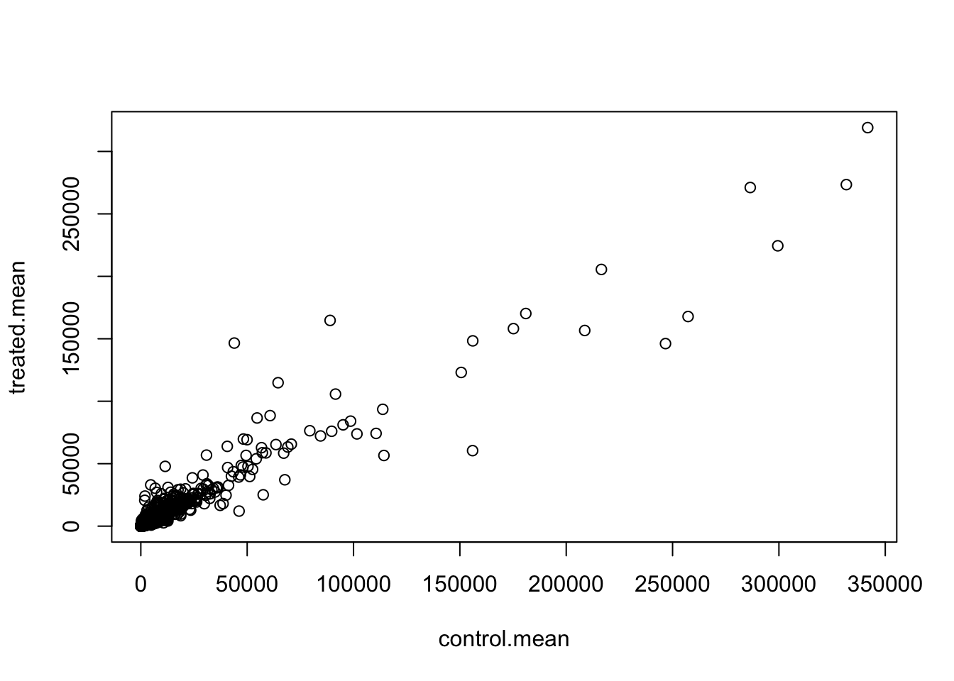
Q5 (b).You could also use the ggplot2 package to make this figure producing the plot below. What geom_?() function would you use for this plot?
library(ggplot2)

ggplot(meancounts, aes(control.mean, treated.mean)) + geom_point(alpha = 0.4)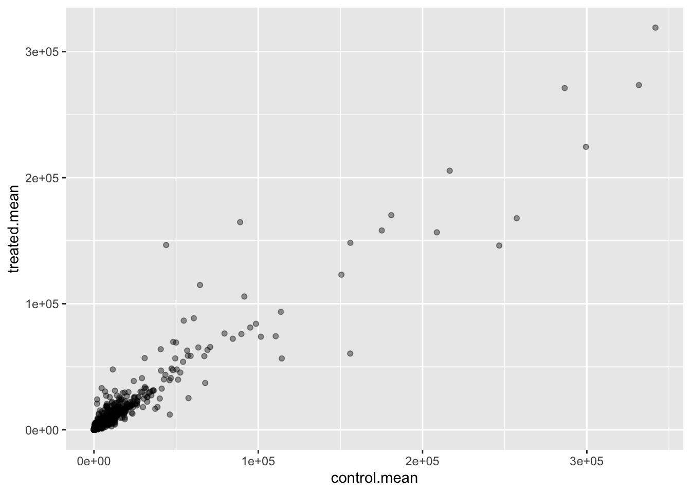
Q6. Try plotting both axes on a log scale. What is the argument to plot() that allows you to do this?
log argument allows to plot both axes on a log scale.
Let’s log transform this count data:
plot(meancounts$control.mean, meancounts$treated.mean, log = "xy", xlab = "log Control", ylab = "log Treated")Warning in xy.coords(x, y, xlabel, ylabel, log): 15032 x values <= 0 omitted
from logarithmic plotWarning in xy.coords(x, y, xlabel, ylabel, log): 15281 y values <= 0 omitted
from logarithmic plot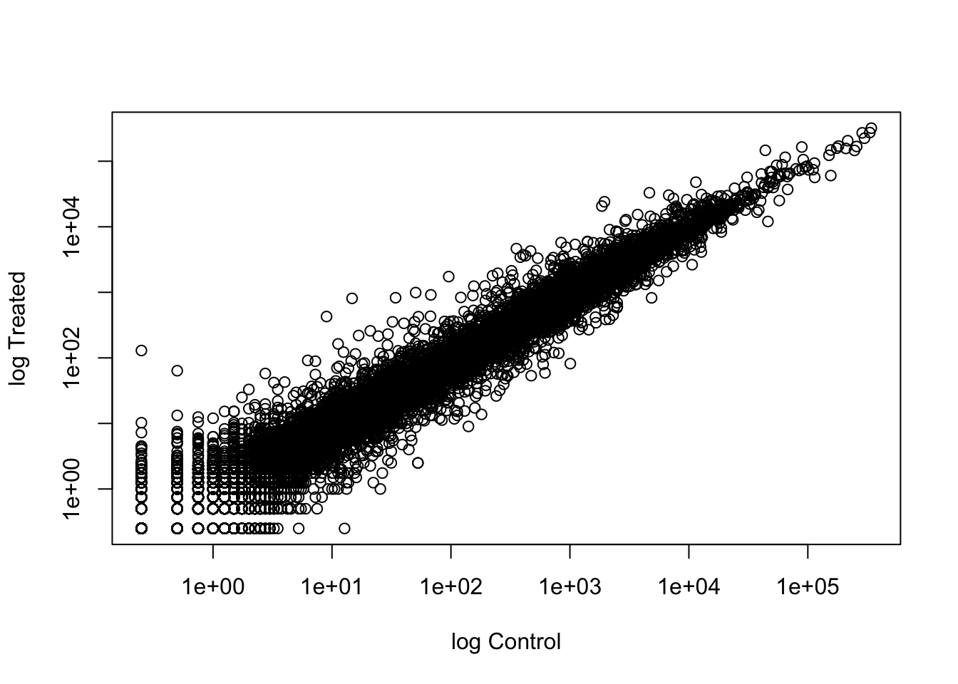
N.B. We most often use log2 for this type of data as it makes the interpretation much more straightforward.
Treated/Control is often called “fold-change”
If there was no change we would have a log2-fc of zero
log2(10/10)[1] 0If we had double the amount of transcript around we would have a log2-fc of 1
log2(20/10)[1] 1If we had half the amount of transcript around we would have a log2-fc of -1
log2(5/10)[1] -1Q. Calculate a log2 fold change value for all our genes and add it as a new column to our
meancountsobject.
meancounts$log2fc <- log2(meancounts$treated.mean/meancounts$control.mean)

head(meancounts)
control.mean treated.mean log2fc
ENSG00000000003 900.75 658.00 -0.45303916
ENSG00000000005 0.00 0.00 NaN
ENSG00000000419 520.50 546.00 0.06900279
ENSG00000000457 339.75 316.50 -0.10226805
ENSG00000000460 97.25 78.75 -0.30441833
ENSG00000000938 0.75 0.00 -InfThere are some “funky” log2fc values (NaN and -Inf) here that come about when ever we have 0 mean count values. Typically we would remove these genes from any further analysis - as we can’t say anything about them if we have no data for them.
zero.vals <- which(meancounts[,1:2]==0, arr.ind=TRUE)

to.rm <- unique(zero.vals[,1])
mycounts <- meancounts[-to.rm,]
head(mycounts)
control.mean treated.mean log2fc
ENSG00000000003 900.75 658.00 -0.45303916
ENSG00000000419 520.50 546.00 0.06900279
ENSG00000000457 339.75 316.50 -0.10226805
ENSG00000000460 97.25 78.75 -0.30441833
ENSG00000000971 5219.00 6687.50 0.35769358
ENSG00000001036 2327.00 1785.75 -0.38194109Q7. What is the purpose of the arr.ind argument in the which() function call above? Why would we then take the first column of the output and need to call the unique() function?
The purpose of the arr.ind argument is to tell us which row and columns have zero counts. Unique() helps us not count a row 2 times if there are zero counts in both control and treated samples.
up.ind <- mycounts$log2fc > 2
down.ind <- mycounts$log2fc < (-2)
Q8. Using the up.ind vector above can you determine how many up regulated genes we have at the greater than 2 fc level?
sum(up.ind)[1] 250Q9. Using the down.ind vector above can you determine how many down regulated genes we have at the greater than 2 fc level?
sum(down.ind)[1] 367Q10. Do you trust these results? Why or why not?
No, these results do not tell us whether the upregulated or downregulated genes are statistically significant. Although a gene could be upregulated, the log fold change could be extremely small, but large enough to pass our manufactured threshold.
DESeq Analysis
Let’s do this analysis with an estimate of statistical significance using the DESeq2 package
library(DESeq2)DESeq (like many bioconductor packages) want it’s input data in a very specific way.
dds <- DESeqDataSetFromMatrix(countData = counts,
                              colData = metadata,
                              design = ~dex)
converting counts to integer modeWarning in DESeqDataSet(se, design = design, ignoreRank): some variables in
design formula are characters, converting to factorsRun the DESeq analysis pipeline
The main function DEseq()
dds <- DESeq(dds)estimating size factorsestimating dispersionsgene-wise dispersion estimatesmean-dispersion relationshipfinal dispersion estimatesfitting model and testingres <- results(dds)
head(res)log2 fold change (MLE): dex treated vs control
Wald test p-value: dex treated vs control
DataFrame with 6 rows and 6 columns
baseMean log2FoldChange lfcSE stat pvalue
<numeric> <numeric> <numeric> <numeric> <numeric>
ENSG00000000003 747.194195 -0.350703 0.168242 -2.084514 0.0371134
ENSG00000000005 0.000000 NA NA NA NA
ENSG00000000419 520.134160 0.206107 0.101042 2.039828 0.0413675
ENSG00000000457 322.664844 0.024527 0.145134 0.168996 0.8658000
ENSG00000000460 87.682625 -0.147143 0.256995 -0.572550 0.5669497
ENSG00000000938 0.319167 -1.732289 3.493601 -0.495846 0.6200029
padj
<numeric>
ENSG00000000003 0.163017
ENSG00000000005 NA
ENSG00000000419 0.175937
ENSG00000000457 0.961682
ENSG00000000460 0.815805
ENSG00000000938 NAAdding Annotation Data
library("AnnotationDbi")
library("org.Hs.eg.db")columns(org.Hs.eg.db) [1] "ACCNUM" "ALIAS" "ENSEMBL" "ENSEMBLPROT" "ENSEMBLTRANS"
[6] "ENTREZID" "ENZYME" "EVIDENCE" "EVIDENCEALL" "GENENAME"
[11] "GENETYPE" "GO" "GOALL" "IPI" "MAP"
[16] "OMIM" "ONTOLOGY" "ONTOLOGYALL" "PATH" "PFAM"
[21] "PMID" "PROSITE" "REFSEQ" "SYMBOL" "UCSCKG"
[26] "UNIPROT" res$symbol <- mapIds(org.Hs.eg.db,
keys=row.names(res), # Our genenames
keytype="ENSEMBL", # The format of our genenames
column="SYMBOL", # The new format we want to add
multiVals="first")'select()' returned 1:many mapping between keys and columnshead(res)log2 fold change (MLE): dex treated vs control
Wald test p-value: dex treated vs control
DataFrame with 6 rows and 7 columns
baseMean log2FoldChange lfcSE stat pvalue
<numeric> <numeric> <numeric> <numeric> <numeric>
ENSG00000000003 747.194195 -0.350703 0.168242 -2.084514 0.0371134
ENSG00000000005 0.000000 NA NA NA NA
ENSG00000000419 520.134160 0.206107 0.101042 2.039828 0.0413675
ENSG00000000457 322.664844 0.024527 0.145134 0.168996 0.8658000
ENSG00000000460 87.682625 -0.147143 0.256995 -0.572550 0.5669497
ENSG00000000938 0.319167 -1.732289 3.493601 -0.495846 0.6200029
padj symbol
<numeric> <character>
ENSG00000000003 0.163017 TSPAN6
ENSG00000000005 NA TNMD
ENSG00000000419 0.175937 DPM1
ENSG00000000457 0.961682 SCYL3
ENSG00000000460 0.815805 FIRRM
ENSG00000000938 NA FGRQ11. Run the mapIds() function two more times to add the Entrez ID and UniProt accession and GENENAME as new columns called res\(entrez, res\)uniprot and res$genename.
res$entrez <- mapIds(org.Hs.eg.db,
                     keys=row.names(res),
                     column="ENTREZID",
                     keytype="ENSEMBL",
                     multiVals="first")
'select()' returned 1:many mapping between keys and columnsres$uniprot <- mapIds(org.Hs.eg.db,
keys=row.names(res),
column="UNIPROT",
keytype="ENSEMBL",
multiVals="first")'select()' returned 1:many mapping between keys and columnsres$genename <- mapIds(org.Hs.eg.db,
keys=row.names(res),
column="GENENAME",
keytype="ENSEMBL",
multiVals="first")'select()' returned 1:many mapping between keys and columnshead(res)log2 fold change (MLE): dex treated vs control
Wald test p-value: dex treated vs control
DataFrame with 6 rows and 10 columns
baseMean log2FoldChange lfcSE stat pvalue
<numeric> <numeric> <numeric> <numeric> <numeric>
ENSG00000000003 747.194195 -0.350703 0.168242 -2.084514 0.0371134
ENSG00000000005 0.000000 NA NA NA NA
ENSG00000000419 520.134160 0.206107 0.101042 2.039828 0.0413675
ENSG00000000457 322.664844 0.024527 0.145134 0.168996 0.8658000
ENSG00000000460 87.682625 -0.147143 0.256995 -0.572550 0.5669497
ENSG00000000938 0.319167 -1.732289 3.493601 -0.495846 0.6200029
padj symbol entrez uniprot
<numeric> <character> <character> <character>
ENSG00000000003 0.163017 TSPAN6 7105 A0A087WYV6
ENSG00000000005 NA TNMD 64102 Q9H2S6
ENSG00000000419 0.175937 DPM1 8813 H0Y368
ENSG00000000457 0.961682 SCYL3 57147 X6RHX1
ENSG00000000460 0.815805 FIRRM 55732 A6NFP1
ENSG00000000938 NA FGR 2268 B7Z6W7
genename
<character>
ENSG00000000003 tetraspanin 6
ENSG00000000005 tenomodulin
ENSG00000000419 dolichyl-phosphate m..
ENSG00000000457 SCY1 like pseudokina..
ENSG00000000460 FIGNL1 interacting r..
ENSG00000000938 FGR proto-oncogene, ..ord <- order( res$padj )
#View(res[ord,])
head(res[ord,])log2 fold change (MLE): dex treated vs control
Wald test p-value: dex treated vs control
DataFrame with 6 rows and 10 columns
baseMean log2FoldChange lfcSE stat pvalue
<numeric> <numeric> <numeric> <numeric> <numeric>
ENSG00000152583 954.771 4.36836 0.2371306 18.4217 8.79214e-76
ENSG00000179094 743.253 2.86389 0.1755659 16.3123 8.06568e-60
ENSG00000116584 2277.913 -1.03470 0.0650826 -15.8983 6.51317e-57
ENSG00000189221 2383.754 3.34154 0.2124091 15.7316 9.17960e-56
ENSG00000120129 3440.704 2.96521 0.2036978 14.5569 5.27883e-48
ENSG00000148175 13493.920 1.42717 0.1003811 14.2175 7.13625e-46
padj symbol entrez uniprot
<numeric> <character> <character> <character>
ENSG00000152583 1.33157e-71 SPARCL1 8404 B4E2Z0
ENSG00000179094 6.10774e-56 PER1 5187 A2I2P6
ENSG00000116584 3.28806e-53 ARHGEF2 9181 A0A8Q3SIN5
ENSG00000189221 3.47563e-52 MAOA 4128 B4DF46
ENSG00000120129 1.59896e-44 DUSP1 1843 B4DRR4
ENSG00000148175 1.80131e-42 STOM 2040 F8VSL7
genename
<character>
ENSG00000152583 SPARC like 1
ENSG00000179094 period circadian reg..
ENSG00000116584 Rho/Rac guanine nucl..
ENSG00000189221 monoamine oxidase A
ENSG00000120129 dual specificity pho..
ENSG00000148175 stomatinVolcano Plot
This is a main summary results figure from these kinds of studies. It is a plot of Log2 fold-change vs (Adjusted) P-Value.
plot(res$log2FoldChange, res$padj)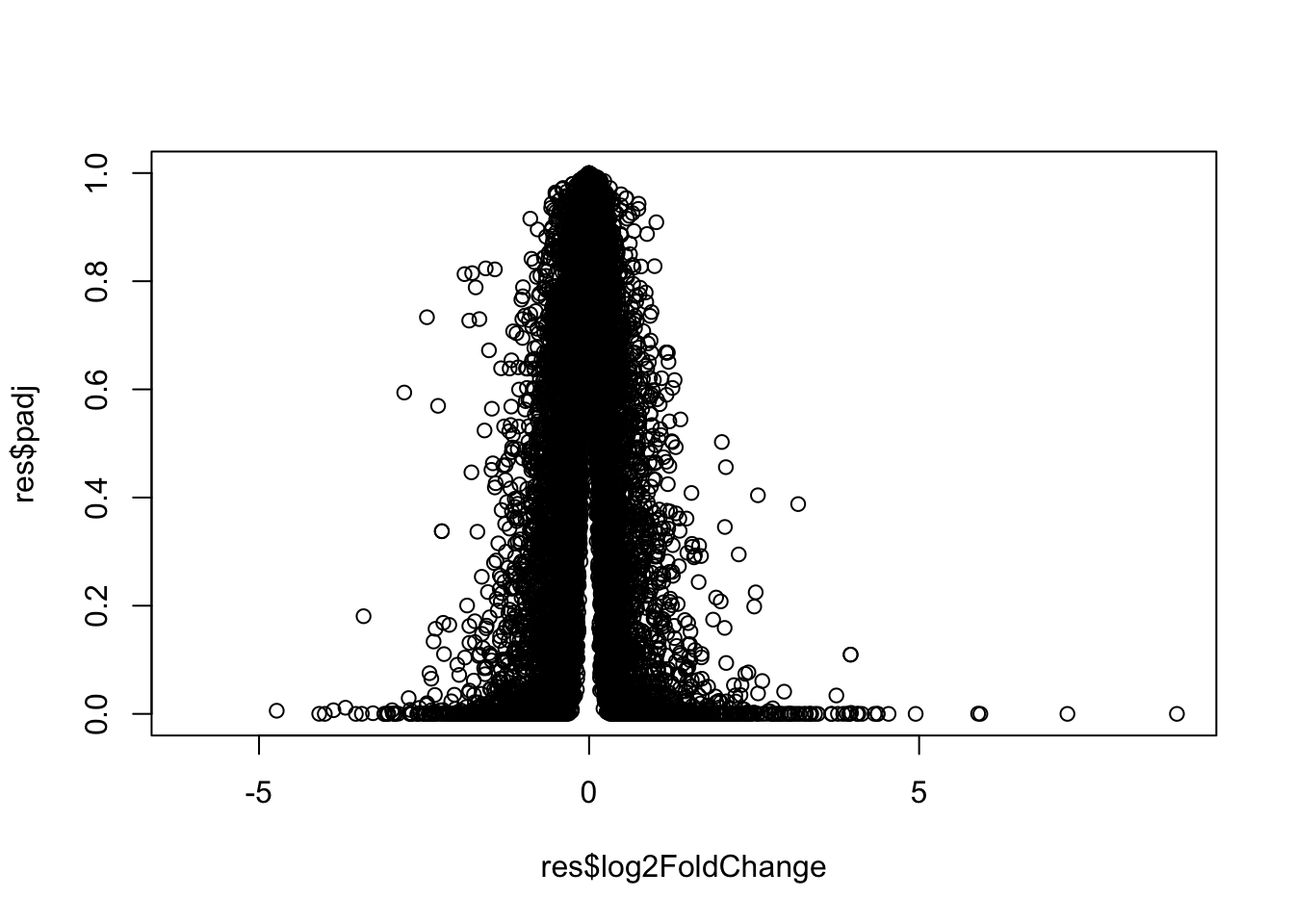
Again this y-axis highly needs log transforming and we can flip the y-axis with a minus sign so it looks like every other vocano plot.
plot(res$log2FoldChange, -log(res$padj))

abline(v=-2, col  = "red")
abline(v=2, col  = "red")
abline(h=-log(0.05), col = "red")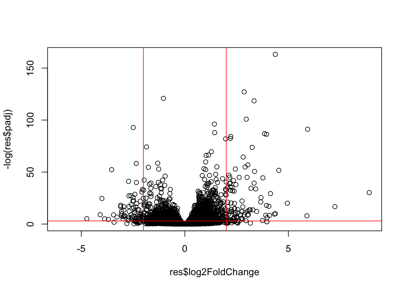
Adding Some Color Annotation
Start with a default base color “gray”
# Custom Colors

# mycols <- "gray"
mycols <- rep("gray", nrow(res))
mycols[res$log2FoldChange > 2] <- "blue"
mycols[res$log2FoldChange < -2] <- "darkgreen"
mycols[res$padj >= 0.05] <- "gray"

# Volcano Plot
plot(res$log2FoldChange, -log(res$padj), col = mycols)

# Cut-off Lines
abline(v=-c(-2,2), col = "gray", lty = 2)
abline(h=-log(0.05), col = "gray", lty = 2)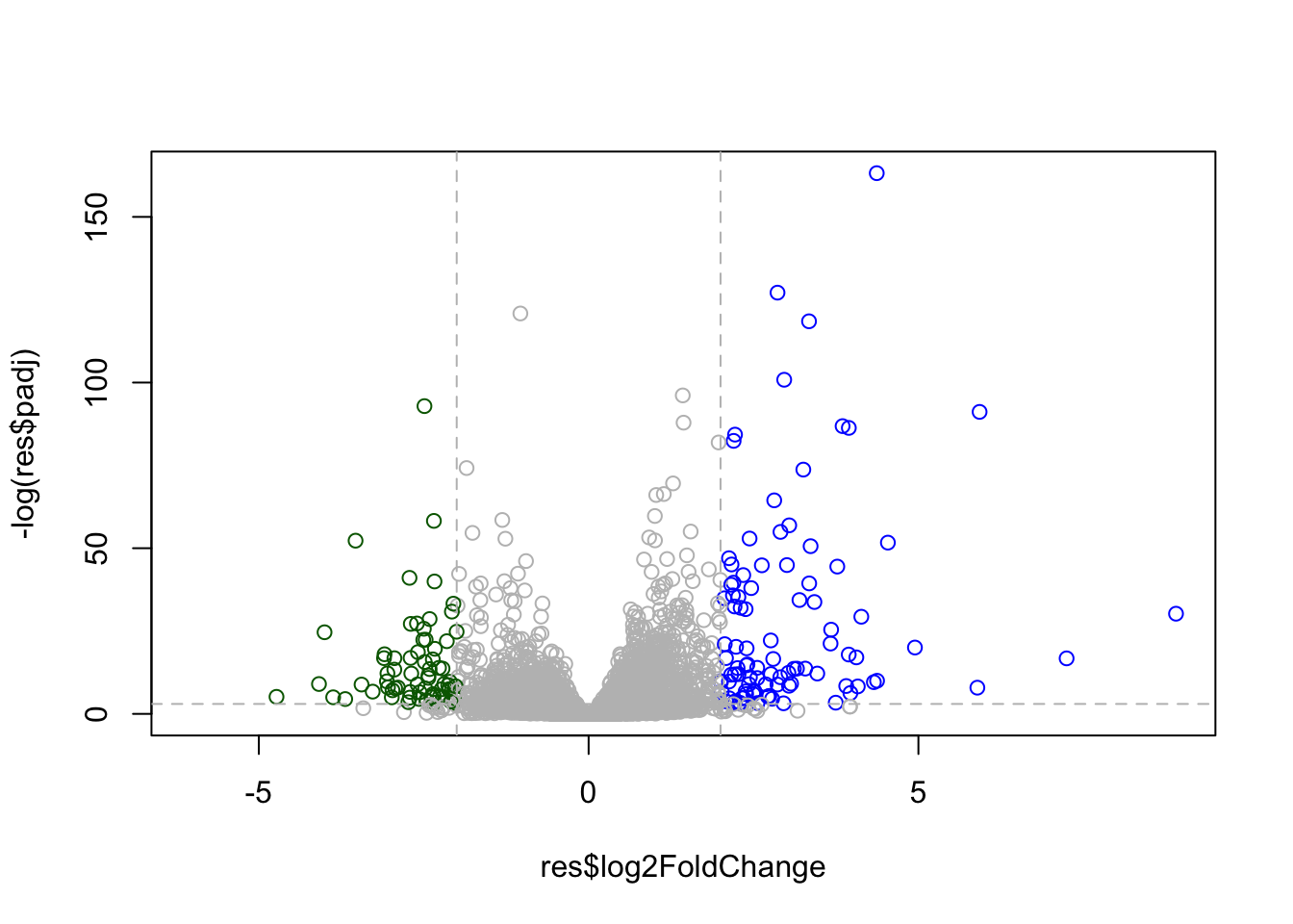
Q. Make a presentation quality ggplot version of this plot. Include clear axis labels, a clean theme, your custom colors, cut-off lines and a plot title.
library(ggplot2)

ggplot(res, aes(log2FoldChange, -log(padj))) +
  geom_point(color = mycols) +
  labs(title = "Volcano Plot of Asthma RNA-Seq Data",
       x = "Log2 Fold-Change",
       y = "-log Adjusted P-Value") +
  geom_hline(yintercept = -log(0.05), color = "darkgray", linetype = "dashed",
             size = 1) +
  geom_vline(xintercept = c(-2,2), color = "darkgray", linetype = "dashed",
             size = 1) +
  theme_bw()
Warning: Using `size` aesthetic for lines was deprecated in ggplot2 3.4.0.
ℹ Please use `linewidth` instead.Warning: Removed 23549 rows containing missing values or values outside the scale range
(`geom_point()`).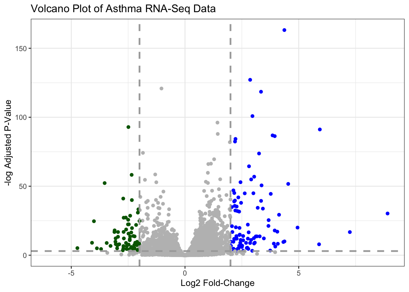
Save our results
Write a CSV file
write.csv(res, file = "results.csv")